

How is a Mondrian painting like a dungeon map?
Abstract art and dungeon layout: an odd couple


First, I wanted to give a big shout out to my first two subscribers:
empirefrizzandishaanksheth. Appreciate your support!
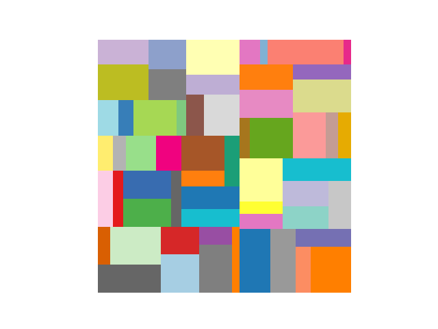
In the early 20th Century, Piet Mondrian, a Dutch artist, was quietly revolutionizing the theory and practice of abstract visual art. While he created art in different styles, he is perhaps best known for his grid-based paintings (see above). These paintings comprise disjoint variegated squares and rectangles filling the entire canvas.
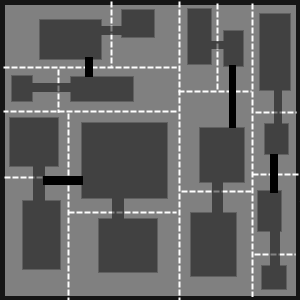
So, how does that relate to dungeon maps? A dungeon layout is a 2D map on a discrete grid indicating which tiles are to be placed in each cell making up the dungeon. In constructing the layout, we need to divide the space into non-overlapping portions, for example, to place rooms and corridors. If we were to divide our space using axis-aligned cuts we would produce a figure (see above) very much like a Mondrian painting.
Binary space partitions
In this article, we’ll look at a simple algorithm to create Mondrian-like “paintings”. Another name for this technique is binary space partitioning. You may have heard of this method in the context of creating an efficient search structure for points in space - an important problem in computer graphics - it’s the same idea.
The algorithm works like so:
Begin with a single cell of the desired final layout size.
Divide the cell along its longest axis, uniformly between
[min_width, width - min_midth]or[min_height, height - min_height], whichever the case may be.Pick a cell at random, and divide it as in Step 2 if its area is greater than
min_area.Repeat Step 3 until there are no dividable cells left.
Here’s an illustration of binary space partitioning in action:
We have design freedom to choose which cell and axis to split at each step, as well as the terminating condition. The parameters are the initial width, height, minimum cell area, minimum cell width and height, and, as always, the random seed.
Implementation
Let’s begin our implementation by defining the data structures for our binary space partition. We represent the partition with a binary tree. The leaves of the tree represent the final partitions of the space, and their ancestor nodes represent intermediate splitting steps:
@dataclass
class Rect:
    x: int = 0
    y: int = 0
    width: int = 0
    height: int = 0

@dataclass
class Node:
    index: int = 0
    rect: Rect = field(default_factory=Rect)
    axis: Optional[int] = None
    split: Optional[int] = None
    left: Optional[”Node”] = None
    right: Optional[”Node”]= None
Each node contains a rectangle describing its area within the layout, references to its left and right child, and we assign it an index for visualization purposes later on. The axis and split fields are optional, but make some parts of the implementation easier.
A binary space partition, then, is represented by a single root node, and, for convenience, we maintain a set of leaf nodes:
class BinarySpacePartition:
    root: Node
    leaves: Set[Node]
The classes initializer sets up the root node and begins splitting:
def __init__(self,
             width: int = 100,
             height: int = 100,
             min_width: int = 10,
             min_height: int = 10,
             min_area: int = 250,
             seed: Optional[int]=None):

    if seed is not None:
        random.seed(seed)

    self.root = Node(index=0)
    self.root.rect = Rect(0, 0, width, height)
    self.axis = 0
    self.count_nodes = 1
    self.leaves = [self.root]

    self._split(min_width, min_height, min_area)
Here is the meat of the code, the splitting algorithm:
def _split(self, min_width: int, min_height: int, min_area: int):
    leaves_todo = list(self.leaves)

    while len(leaves_todo):
        candidate = random.choice(leaves_todo)
        leaves_todo.remove(candidate)

        # Work out whether we need to split this node
        r = candidate.rect
        if (min_area < r.width * r.height):
            # Split maximum dimension
            if r.width > r.height:
                candidate.axis = 0
            else:
                candidate.axis = 1

        if candidate.axis == 0:
            candidate.split = random.randrange( \
                min(min_width, r.width - min_width), \
                max(r.width - min_width, min_width) + 1)

            candidate.left = Node( \
                index=candidate.index, \
                rect=Rect(r.x, r.y, candidate.split, r.height))

            candidate.right = Node( \
                index=len(self.leaves), \
                rect=Rect(r.x + candidate.split, r.y, \
                          r.width - candidate.split, r.height))

        else:
            candidate.split = random.randrange( \
                min(min_height, r.height - min_height), \
                max(r.height - min_height, min_height) + 1)

            candidate.left = Node(index=candidate.index, \
                rect=Rect(r.x, r.y, r.width, candidate.split))

            candidate.right = Node( \
                index=len(self.leaves), \
                rect=Rect(r.x, r.y + candidate.split,
                          r.width, r.height - candidate.split))

        # Update leaves
        self.leaves.remove(candidate)
        self.leaves.extend([candidate.left, candidate.right])
        leaves_todo.extend([candidate.left, candidate.right])
An animation of this algorithm was given in the previous section. The end result is a layout like this:
Discussion
In implementing the algorithm in Python from scratch, I discovered some gotchas that seem obvious after the fact.
In my first implementation attempt, I performed the splits in a depth-first manner. This produces similar output to the final method I decided upon but doesn’t nearly look as good for visualization. Also, choosing which cell to split at random allows additional termination conditions, such as: “conclude when there are x cells” (and the layout will be balanced).
For the termination condition, I began with a rule that terminated when neither axis of a cell could be split so that the width or height would be greater than some minimum threshold. However, this resulted in too many square-like cells rather than a diversity of aspect ratios.
Some alternatives I tried for choosing which axis to split were:
choose the axis at random; and.
alternate the axis to split from parent to child.
These produced reasonable results, although contained many cells that were too long in one axis. Better results, in my (subjective) opinion, achieve a sweet spot for the distribution of cell aspect ratios. We don’t want them all to be square-like, but neither do we want them to be long and skinny.
These observations drove home the message that procedural generation is part science, part art. We have to implement the methods with an understanding of the constraints that make the output believable, interesting, and fun.
What’s next?
One method to use a binary space partition to construct a dungeon layout, is to place a room in each cell. The room can be smaller than the cell and offset randomly from the cell boundary. Then we can simply join adjacent cells in some way:
Being able to construct a binary space partition, however, is a very general purpose tool for dividing the layout space and can be combined effectively with other methods.
In my next post, we’ll continue our discussion of traditional PCG methods for dungeon building with another method that achieves a disjoint partition but without aligning the splits to the axes.
Resources
Full Python implementation (to be posted shortly): https://github.com/stefanwebb/generative-gamedev